Exploring Network Models
Previous post: Creating a Network Graph
There are a number of definitions for what it means to belong to a community. Usually, people are involved in multiple communities, but they have stronger ties to a few of those communities because they know more people in those communities than in the others. In terms of graph theory, a community has a more specific definition: a community is a subgraph where “the number of internal edges is larger than the number of external edges” (Fortunato and Hric 2016). The internal edges are the links that connect together nodes inside the subgraph, while external edges refer to the links that connect nodes inside the subgraph to nodes outside the subgraph. Within this definition of community, there are two types: strong communities and weak communities. A strong community is one where every node in the community has more internal edges than external edges. A weak community is simply one where the total number of all nodes’ internal edges is larger than the total number of their external edges. In this context, it can be easier to think of a strong community as a specific form of weak community. In other words, a strong community is also a weak community, but not all weak communities are strong communities (Fortunato and Hric 2016). But this definition is based on the classic network science view of communities, where edge counting and centrality-based measures define relationships. It also implies that communities are usually well separated from each other in the graph, which is not always the case. In this post, we’ll take a look at two common community-detection algorithms as well as a new vector-based algorithm in order to compare and contrast the communities found.
Girvan-Newman
One classic algorithm we tested was Girvan-Newman (GN). It finds communities by progressively removing edges from the original graph. At each step, it looks at the betweenness centrality of each node and then removes the edge with the highest betweenness score. It repeats this until there are no more edges with the highest score. The remaining connected components are the communities. In other words, instead of looking for edges that are more likely to be in a community, it looks for edges to remove in between communities (Girvan and Newman, 2002). Using the bipartite graph we made, we used a Python library called igraph and found 23 communities.
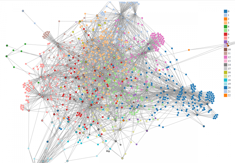
The entire graph colored by Girvan Newman partitions. The nodes with a black border represent documents.
The code for this visualization can be found here.
To determine how well the algorithm separated the nodes into groups, we used a measure called modularity. Modularity is “the fraction of the edges that fall within the given groups minus the expected fraction if edges were distributed at random.” The range of values fall between -1 and 1 (Li and Schuurmans, 2011). The modularity score for GN was ~0.519, which seems to reflect the fact that it had some trouble separating the graph into communities. Graphs with high modularity scores usually have nodes grouped into several strong communities. In this case, the nodes were not as well separated.
Within the communities that were found, many nodes were grouped based on the states and cities of the documents, which was not surprising given that the document nodes had the highest betweenness values. Some interesting communities were:
- 3 (mostly NY, but CT, MD, and MA appeared)
- 5 (MA, NY, PA, NJ)
- 17 & 18 (NY, PA, and DC, 18: CT added)
- 20 (NY and MD)
- 19 (majority NC but outliers TN and PA)
- 6 (TN, KY, MI)
- 15 (TX and Ontario, Canada)
The first four communities were mostly regional in the Northeast but touched a few Mid-Atlantic states. Then in 19, the communities spread into the South with TN and NC. However, the direction of the spread of influence is difficult to perceive since the date is only mentioned on the label of the document node, and label names do not affect the algorithm. We see more vertical geographic spreading at 6 and 15. While 6 can be connected to the spread from 19, 15 seems to be completely independent of the rest of the communities.
For those interested, our code for this analysis can be found here underneath Girvan-Newman.
Louvain
The second algorithm that is computationally faster than GN is Louvain. It uses modularity as a heuristic to group nodes efficiently. Usually, we would have to observe all the possible ways in which nodes can be grouped together. However, the runtime can be very inefficient as finding all possible ways would grow exponentially with the number of nodes. Louvain uses modularity as a shortcut to group nodes locally until the modularity can’t be measured anymore. This works in two phases. In the first phase, each node in the graph is assigned its own community and modularities. For example, suppose there are 20 nodes in a connected graph, then each node will be assigned by its own community by a numerical label such as node 0 belonging to 0, node 1 belonging to 1, etc. Additionally, the algorithm traverses through the nodes sequentially, the nodes themselves are not “ordered” by a label.
Afterward, the algorithm removes the node from its own community and moves into each of its neighbors. During this move, it calculates the difference in modularity. The selected node is then placed in a neighboring community according to the maximum modularity difference. If the change is not possible, then the node remains in its own community. This is repeated for every node in the graph until the algorithm cannot calculate the change anymore.
In the second phase, it creates a new graph where each node represents each new community from the first phase. Any node from the first phase that shares different communities is a weighted edge between two community nodes in this graph. Then, we re-use this graph to repeat the first phase again until there is no community node left (Blondel et. al., 2008).
We found 11 communities, which was half as many communities found in GN. However, the modularity score was around the same as GN, with the value of ~0.511. Although optimizing community through maximizing modularity was supposed to find better communities, this did not have an effect on a larger bipartite network. Louvain also clustered graphs by regions, such as:
- 0: all NY cities
- 1: all PA cities
- 5: IN and OH cities, with 1 KS and 1 PA city.
However, there were a few interesting groups that showed vertical translation, such as
- 2: MA and KS.
- 6: ON (Ontario, Canada) and TX
Additionally, Kansas is involved with 2 and 6 in different documents with one person in common from the original adjacency list and GN subgraph 16. However, this person was not mentioned in group 6 here.
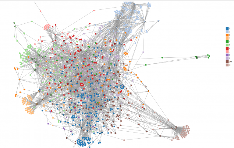
The same graph colored by Louvain partitions.
The d3 code for the visualization can be found here, as well as the Python code here underneath Louvain.
Node2vec
Lastly, we tested community detection with a vector-based model called node2vec. Although node2vec is a more generic version of word2vec, it can also be used to cluster nodes and detect communities. Node2vec achieves this in two phases: sampling, then embedding.
Embedding is mapping any object into a vector with real numbers. In word2vec, it maps a word into an n-dimensional vector. It uses the skip-gram model, which is a simple neural network with one hidden layer and the input is sentences. We train the neural network to find probabilities of every word in the given vocabulary of being the “nearest word” for the selected word in the sentence. Then, the output layer is removed to reveal the hidden layer, which contains the vectors for each word in the vocab. However, the skip-gram model requires sentences as input. How do we “sample” sentences from a graph?
We mimic sentences by sampling all possible directed acyclical graphs (DAGs) in the graph. In other words, we find paths that go in one direction from every node. Two important parameters we can set are the length of the path and the number of paths to find from each node. The other two parameters, p and q, determine how we explore our paths. Suppose the algorithm recently transitioned from node t to node v in the picture below [put picture]. P controls the probability to go back to visiting t, while Q controls the probability to visit v’s unvisited neighbors. After sampling all possible DAGs, we can then use them for our skip-gram model to embed the nodes. Additionally, we can also give the number of dimensions as an argument for the skip-gram model.
In node2vec, it was a little difficult to determine exactly how many communities we found. Visually, it can be discerned that about 8 – 10 clusters are found. A few calls to the most_similar function found similar nodes with only last names, which may help in finding duplicate nodes from our first post in NER tagging. Other calls did seem to link to groups of people, although when crossed-referenced with the Louvain and GN groups, some names were not in the cluster at all. We may have to tweak our length to be a little shorter to find more relative groups. In Grover and Leskovec’s original paper for node2vec, the community detection was conducted on the Les Miserables character co-occurrence matrix[cite]. Our current graph’s people nodes are not connected to each other. They can only be connected to document nodes. Therefore, our node2vec model grouped nodes according to the document’s region, similar to GN and Louvain. In the t-SNE plot, you can see that a cluster of people nodes (blue) was often close to at least 1 document node (red) here on the last cell of this notebook.
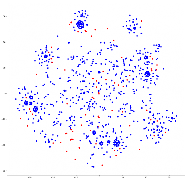
These are the node2vec clusters mapped in 2 dimensions by TSNE.
Analysis
In terms of actually separating communities well, it seems that Louvain and GN performed the same according to modularity. As for the communities themselves, both Louvain and GN show vertical and lateral movement, although fewer communities do not necessarily mean better-structured communities, because modularity may be an inaccurate measure of how communities are constructed. Firstly, modularity is solely based on the number of edges in the graph. This can cause a few problems. Firstly, if the graph is completely random with no labeled groups, the algorithms can still find non-existent communities. Secondly, suppose we generated all randomizations of groups in a graph, and in most versions, subgraphs A and B usually aren’t connected. A single edge between these two can make the combined modularity larger than their own modularities separately. In other words, A and B combined are more likely to be identified as a community than they are separated in most randomizations. This means that modularity favors communities with more edges than analyzing the actual structure of the community in comparison to the rest of the graph. This could be troublesome if the size of actual communities doesn’t have anything to do with the number of edges within them (Fortunato and Hric, 2016).
Node2vec gave us similar groupings, but this is mostly due to the structure of the graph which is bipartite, as opposed to the co-occurrence graph in Les Miserables in the original paper. The vectors for each node seemed helpful, but we have yet to understand how to manipulate the given parameters. There are many given to us, but one clue from the original paper is that by setting p to 1 and q to 0.5, this can mimic a breadth-first search within the sampling technique to find communities. Additionally, the number of dimensions in word2vec is usually the size of its vocabulary or the number of all words ever. Therefore, we can set the dimensions as the number of all nodes in the graph. First, we would need to add edges between the people that co-occur in all documents, even if they attend more than one conference. Then, we can test the parameters walking length and number of paths.
If you’ve ever had experience working with node2vec, leave a comment down below! Tune in soon for our last post!